Suppose Cr11 is the Vector Space of Continuous Realvalued Functions Show That U Perp 0

5 Vector Space $\mathbb{R}^n$

In Section 2.2 we introduced the set $\mathbb{R}^n$ of all $n$ -tuples (called \textit{vectors}), and began our investigation of the matrix transformations $\mathbb{R}^n$ $\to$ $\mathbb{R}^m$ given by matrix multiplication by an $m \times n$ matrix. Particular attention was paid to the euclidean plane $\mathbb{R}^2$ where certain simple geometric transformations were seen to be matrix transformations.

In this chapter we investigate $\mathbb{R}^n$ in full generality, and introduce some of the most important concepts and methods in linear algebra. The $n$ -tuples in $\mathbb{R}^n$ will continue to be denoted $\vec{x}$ , $\vec{y}$ , and so on, and will be written as rows or columns depending on the context.

Subspaces of $\mathbb{R}^n$

We say that the subset $U$ is closed under addition if S2 holds, and that $U$ is closed under scalar multiplication if S3 holds.

Clearly $\mathbb{R}^n$ is a subspace of itself, and this chapter is about these subspaces and their properties. The set $U = \{\vec{0}\}$ , consisting of only the zero vector, is also a subspace because $\vec{0} + \vec{0} = \vec{0}$ and $a\vec{0} = \vec{0}$ for each $a$ in $\mathbb{R}$ ; it is called the zero subspace. Any subspace of $\mathbb{R}^n$ other than $\{\vec{0}\}$ or $\mathbb{R}^n$ is called a proper subspace.

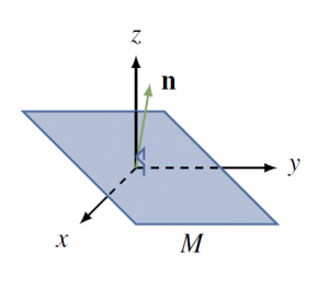A plane We saw in Section 4.2 that every plane $M$ through the origin in $\mathbb{R}^3$ has equation $ax + by + cz = 0$ where $a$ , $b$ , and $c$ are not all zero. Here $\vec{n} = \left[ \begin{array}{r} a \\ b \\ c \end{array} \right]$ is a normal for the plane and

$\begin{equation*} M = \{ \vec{v} \mbox{ in }\mathbb{R}^3 \mid \vec{n} \cdot \vec{v} = 0 \} \end{equation*}$

where
$\vec{v} = \left[ \begin{array}{r} x \\ y \\ z \end{array} \right]$ and $\vec{n} \cdot \vec{v}$ denotes the dot product introduced in Section 2.2 (see the diagram). Then $M$ is a subspace of $\RR^3$ . Indeed we show that $M$ satisfies S1, S2, and S3 as follows:

S1. $\vec{0} \in M$ because $\vec{n} \cdot \vec{0} = 0$ ;

S2. If $\vec{v} \in M$ and $\vec{v}_{1} \in M$ , then $\vec{n} \cdot (\vec{v} + \vec{v}_{1}) = \vec{n} \cdotprod \vec{v} + \vec{n} \cdot \vec{v}_{1} = 0 + 0 = 0$ , so $\vec{v} + \vec{v}_{1} \in M$ ;

S3. If $\vec{v} \in M$ , then $\vec{n} \cdot (a\vec{v}) = a(\vec{n} \cdot \vec{v}) = a(0) = 0$ , so $a\vec{v} \in M$ .

Planes and lines through the origin in $\mathbb{R}^3$ are all subspaces of $\mathbb{R}^3$ .

Solution:

We proved the statement for planes above. If $L$ is a line through the origin with direction vector $\vec{d}$ , then $L = \{t\vec{d} \mid t \in \mathbb{R}\}$ . Can you verify that $L$ satisfies S1, S2, and S3?

Example 5.1.1 shows that lines through the origin in $\mathbb{R}^2$ are subspaces; in fact, they are the only proper subspaces of $\mathbb{R}^2$ . Indeed, we will prove that lines and planes through the origin in $\mathbb{R}^3$ are the only proper subspaces of $\mathbb{R}^3$ . Thus the geometry of lines and planes through the origin is captured by the subspace concept. (Note that every line or plane is just a translation of one of these.)

Subspaces can also be used to describe important features of an $m \times n$ matrix $A$ . The null space of $A$ , denoted $\func{null} A$ , and the image space of $A$ , denoted $\func{im} A$ , are defined by

$\begin{equation*} \func{null } A = \{ \vec{x} \in \mathbb{R}^n \mid A\vec{x} = \vec{0}\} \quad \mbox{ and } \quad \func{im } A = \{A\vec{x} \mid \vec{x} \in \mathbb{R}^n\} \end{equation*}$

In the language of Chapter 2, $\func{null} A$ consists of all solutions $\vec{x}$ in $\mathbb{R}^n$ of the homogeneous system $A\vec{x} = \vec{0}$ , and $\func{im} A$ is the set of all vectors $\vec{y}$ in $\mathbb{R}^m$ such that $A\vec{x} = \vec{y}$ has a solution $\vec{x}$ . Note that $\vec{x}$ is in $\func{null} A$ if it satisfies the condition $A\vec{x} = \vec{0}$ , while $\func{im} A$ consists of vectors of the form $A\vec{x}$ for some $\vec{x}$ in $\mathbb{R}^n$ . These two ways to describe subsets occur frequently.

Solution:

The zero vector $\vec{0} \in \mathbb{R}^n$ lies in $\func{null} A$ because $A\vec{0} = \vec{0}$ . If $\vec{x}$ and $\vec{x}_{1}$ are in $\func{null} A$ , then $\vec{x} + \vec{x}_{1}$ and $a\vec{x}$ are in $\func{null} A$ because they satisfy the required condition:
$\begin{equation*} A(\vec{x} + \vec{x}_1) = A\vec{x} + A\vec{x}_1 = \vec{0} + \vec{0} = \vec{0} \quad \mbox{and} \quad A(a\vec{x}) = a(A\vec{x}) = a\vec{0} = \vec{0} \end{equation*}$

Hence $\func{null} A$ satisfies S1, S2, and S3, and so is a subspace of $\mathbb{R}^n$ .
The zero vector $\vec{0} \in \mathbb{R}^m$ lies in $\func{im} A$ because $\vec{0} = A\vec{0}$ . Suppose that $\vec{y}$ and $\vec{y}_{1}$ are in $\func{im} A$ , say $\vec{y} = A\vec{x}$ and $\vec{y}_{1} = A\vec{x}_{1}$ where $\vec{x}$ and $\vec{x}_{1}$ are in $\mathbb{R}^n$ . Then
$\begin{equation*} \vec{y} + \vec{y}_1 = A\vec{x} + A\vec{x}_1 = A(\vec{x} + \vec{x}_1) \quad \mbox{and} \quad a\vec{y} = a(A\vec{x}) = A(a\vec{x}) \end{equation*}$

show that $\vec{y} + \vec{y}_{1}$ and $a\vec{y}$ are both in $\func{im} A$ (they have the required form). Hence $\func{im} A$ is a subspace of $\mathbb{R}^m$ .

There are other important subspaces associated with a matrix $A$ that clarify basic properties of $A$ . If $A$ is an $n \times n$ matrix and $\lambda$ is any number, let

$\begin{equation*} E_\lambda(A) = \{\vec{x} \in \mathbb{R}^n \mid A\vec{x} = \lambda\vec{x} \} \end{equation*}$

A vector $\vec{x}$ is in $E_\lambda(A)$ if and only if $(\lambda I - A)\vec{x} = \vec{0}$ , so Example 5.1.2 gives:

$E_\lambda(A)$ is called the eigenspace of $A$ corresponding to $\lambda$ . The reason for the name is that, in the terminology of Section 3.3, $\lambda$ is an eigenvalue of $A$ if $E_\lambda(A) \neq \{\vec{0}\}$ . In this case the nonzero vectors in $E_\lambda(A)$ are called the eigenvectors of $A$ corresponding to $\lambda$ .

The reader should not get the impression that every subset of $\mathbb{R}^n$ is a subspace. For example:

$\begin{align*} U_1 &= \left \{ \left[ \begin{array}{l} x \\ y \end{array} \right] \, \middle| \, x \geq 0 \right\} \mbox{ satisfies S1 and S2, but not S3;} \\ U_2 &= \left \{ \left[ \begin{array}{l} x \\ y \end{array} \right] \, \middle| \, x^2 = y^2 \right\} \mbox{ satisfies S1 and S3, but not S2;} \end{align*}$

Hence neither $U_{1}$ nor $U_{2}$ is a subspace of $\RR^2$ .

Spanning sets

Let $\vec{v}$ and $\vec{w}$ be two nonzero, nonparallel vectors in $\mathbb{R}^3$ with their tails at the origin. The plane $M$ through the origin containing these vectors is described in Section 4.2 by saying that $\vec{n} = \vec{v} \times \vec{w}$ is a normal for $M$ , and that $M$ consists of all vectors $\vec{p}$ such that $\vec{n} \cdot\vec{p} = 0$ .
While this is a very useful way to look at planes, there is another approach that is at least as useful in $\mathbb{R}^3$ and, more importantly, works for all subspaces of $\mathbb{R}^n$ for any $n \geq 1$ .

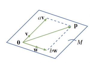Spanning set The idea is as follows: Observe that, by the diagram, a vector $\vec{p}$ is in $M$ if and only if it has the form

$\begin{equation*} \vec{p} = a\vec{v} + b\vec{w} \end{equation*}$

for certain real numbers $a$ and $b$ (we say that $\vec{p}$ is a linear combination of $\vec{v}$ and $\vec{w}$ ).
Hence we can describe $M$ as

$\begin{equation*} M = \{a\vec{x} + b\vec{w} \mid a, b \in \mathbb{R} \} \end{equation*}$

and we say that $\{\vec{v}, \vec{w}\}$ is a spanning set for $M$ . It is this notion of a spanning set that provides a way to describe all subspaces of $\mathbb{R}^n$ .

As in Section 1.3, given vectors $\vec{x}_{1}, \vec{x}_{2}, \dots, \vec{x}_{k}$ in $\mathbb{R}^n$ , a vector of the form

$\begin{equation*} t_1\vec{x}_1 + t_2\vec{x}_2 + \dots + t_k\vec{x}_k \quad \mbox{where the } t_i \mbox{ are scalars} \end{equation*}$

is called a linear combination of the $\vec{x}_{i}$ , and $t_{i}$ is called the coefficient of $\vec{x}_{i}$ in the linear combination.

Here are two examples:

$\begin{equation*} \func{span}\{ \vec{x} \} = \{t\vec{x} \mid t \in \mathbb{R}\} \end{equation*}$

which we write as $\func{span}\{\vec{x}\} = \mathbb{R} \vec{x}$ for simplicity.

$\begin{equation*} \func{span}\{\vec{x}, \vec{y}\} = \{r\vec{x} + s\vec{y} \mid r, s \in \mathbb{R} \} \end{equation*}$

In particular, the above discussion shows that, if $\vec{v}$ and $\vec{w}$ are two nonzero, nonparallel vectors in $\mathbb{R}^3$ , then

$\begin{equation*} M = \func{span}\{\vec{v}, \vec{w} \} \end{equation*}$

is the plane in $\mathbb{R}^3$ containing $\vec{v}$ and $\vec{w}$ . Moreover, if $\vec{d}$ is any nonzero vector in $\mathbb{R}^3$ (or $\mathbb{R}^2$ ), then

$\begin{equation*} L = \func{span} \{\vec{v}\} = \{t\vec{d} \mid t \in \mathbb{R}\} = \mathbb{R}\vec{d} \end{equation*}$

is the line with direction vector $\vec{d}$ . Hence lines and planes can both be described in terms of spanning sets.

Solution:

The vector $\vec{p}$ is in $U$ if and only if $\vec{p} = s\vec{x} + t\vec{y}$ for scalars $s$ and $t$ . Equating components gives equations

$\begin{equation*} 2s + 3t = 0, \quad -s + 4t = -11, \quad 2s - t = 8, \quad \mbox{and} \quad s + t = 1 \end{equation*}$

This linear system has solution $s = 3$ and $t = -2$ , so $\vec{p}$ is in $U$ . On the other hand, asking that $\vec{q} = s\vec{x} + t\vec{y}$ leads to equations

$\begin{equation*} 2s + 3t = 2, \quad -s +4t = 3, \quad 2s -t = 1, \quad \mbox{and} \quad s + t = 2 \end{equation*}$

and this system has no solution. So $\vec{q}$ does not lie in $U$ .

Proof:

The zero vector $\vec{0}$ is in $U$ because $\vec{0} = 0\vec{x}_{1} + 0\vec{x}_{2} + \dots + 0\vec{x}_{k}$ is a linear combination of the $\vec{x}_{i}$ . If $\vec{x} = t_{1}\vec{x}_{1} + t_{2}\vec{x}_{2} + \dots + t_{k}\vec{x}_{k}$ and $\vec{y} = s_{1}\vec{x}_{1} + s_{2}\vec{x}_{2} + \dots + s_{k}\vec{x}_{k}$ are in $U$ , then $\vec{x} + \vec{y}$ and $a\vec{x}$ are in $U$ because
$\begin{eqnarray*} \vec{x} + \vec{y} &=& (t_1 + s_1)\vec{x}_1 + (t_2 + s_2)\vec{x}_2 + \dots + (t_k + s_k)\vec{x}_k, \mbox{ and} \\ a\vec{x} &=& (at_1)\vec{x}_1 + (at_2)\vec{x}_2 + \dots + (at_k)\vec{x}_k \end{eqnarray*}$

Finally each $\vec{x}_i$ is in $U$ (for example, $\vec{x}_2 = 0\vec{x}_1 + 1\vec{x}_2 + \dots + 0\vec{x}_k$ ) so S1, S2, and S3 are satisfied for $U$ , proving (1).
Let $\vec{x} = t_{1}\vec{x}_{1} + t_{2}\vec{x}_{2} + \dots + t_{k}\vec{x}_{k}$ where the $t_{i}$ are scalars and each $\vec{x}_{i} \in W$ . Then each $t_{i}\vec{x}_{i} \in W$ because $W$ satisfies S3. But then $\vec{x} \in W$ because $W$ satisfies S2 (verify). This proves (2).

Condition (2) in Theorem 5.1.1 can be expressed by saying that $\func{span}\{\vec{x}_{1}, \vec{x}_{2}, \dots, \vec{x}_{k}\}$ is the smallest subspace of $\mathbb{R}^n$ that contains each $\vec{x}_{i}$ . This is useful for showing that two subspaces $U$ and $W$ are equal, since this amounts to showing that both $U \subseteq W$ and $W \subseteq U$ . Here is an example of how it is used.

Solution:

Since both $\vec{x} + \vec{y}$ and $\vec{x} - \vec{y}$ are in $\func{span}\{\vec{x}, \vec{y}\}$ , Theorem 5.1.1 gives

$\begin{equation*} \func{span}\{\vec{x} + \vec{y}, \vec{x} - \vec{y} \} \subseteq \func{span}\{\vec{x}, \vec{y}\} \end{equation*}$

But $\vec{x} = \frac{1}{2}(\vec{x} + \vec{y}) + \frac{1}{2}(\vec{x} - \vec{y})$ and $\vec{y} = \frac{1}{2}(\vec{x} + \vec{y}) - \frac{1}{2}(\vec{x} - \vec{y})$ are both in $\func{span}\{\vec{x} + \vec{y}, \vec{x} - \vec{y}\}$ , so

$\begin{equation*} \func{span}\{\vec{x}, \vec{y}\} \subseteq \func{span}\{\vec{x} + \vec{y}, \vec{x} - \vec{y} \} \end{equation*}$

again by Theorem 5.1.1. Thus $\func{span}\{\vec{x}, \vec{y}\} = \func{span}\{\vec{x} + \vec{y}, \vec{x} - \vec{y}\}$ , as desired.

It turns out that many important subspaces are best described by giving a spanning set. Here are three examples, beginning with an important spanning set for $\mathbb{R}^n$ itself. Column $j$ of the $n \times n$ identity matrix $I_{n}$ is denoted $\vec{e}_{j}$ and called the $j$ th coordinate vector in $\mathbb{R}^n$ , and the set $\{\vec{e}_{1}, \vec{e}_{2}, \dots, \vec{e}_{n}\}$ is called the standard basis of $\mathbb{R}^n$ . If
$\vec{x} = \left[ \begin{array}{r} x_1 \\ x_2 \\ \vdots \\ x_n \end{array} \right]$ is any vector in $\mathbb{R}^n$ , then $\vec{x} = x_{1}\vec{e}_{1} + x_{2}\vec{e}_{2} + \dots + x_{n}\vec{e}_{n}$ , as the reader can verify. This proves:

If $A$ is an $m \times n$ matrix $A$ , the next two examples show that it is a routine matter to find spanning sets for $\func{null} A$ and $\func{im} A$ .

Solution:

If $\vec{x} \in \func{null} A$ , then $A\vec{x} = \vec{0}$ so Theorem 1.3.2 shows that $\vec{x}$ is a linear combination of the basic solutions; that is, $\func{null} A \subseteq \func{span}\{\vec{x}_{1}, \vec{x}_{2}, \dots, \vec{x}_{k}\}$ . On the other hand, if $\vec{x}$ is in $\func{span}\{\vec{x}_{1}, \vec{x}_{2}, \dots, \vec{x}_{k}\}$ , then $\vec{x} = t_{1}\vec{x}_{1} + t_{2}\vec{x}_{2} + \dots + t_{k}\vec{x}_{k}$ for scalars $t_{i}$ , so

$\begin{equation*} A\vec{x} = t_1A\vec{x}_1 + t_2A\vec{x}_2 + \dots + t_kA\vec{x}_k = t_1\vec{0} + t_2\vec{0} + \dots + t_k\vec{0} = \vec{0} \end{equation*}$

This shows that $\vec{x} \in \func{null} A$ , and hence that $\func{span}\{\vec{x}_{1}, \vec{x}_{2}, \dots, \vec{x}_{k}\} \subseteq \func{null} A$ . Thus we have equality.

Let $\vec{c}_{1}, \vec{c}_{2}, \dots, \vec{c}_{n}$ denote the columns of the $m \times n$ matrix $A$ . Then

$\begin{equation*} \func{im } A = \func{span}\{\vec{c}_1, \vec{c}_2, \dots, \vec{c}_n\} \end{equation*}$

Solution:

If $\{\vec{e}_{1}, \vec{e}_{2}, \dots, \vec{e}_{n}\}$ is the standard basis of $\mathbb{R}^n$ , observe that

$\begin{equation*} \left[ \begin{array}{cccc} A\vec{e}_1 & A\vec{e}_2 & \cdots & A\vec{e}_n \end{array}\right] = A \left[ \begin{array}{cccc} \vec{e}_1 & \vec{e}_2 & \cdots & \vec{e}_n \end{array}\right] = AI_n = A = \left[ \begin{array}{cccc} \vec{c}_1 & \vec{c}_2 & \cdots \vec{c}_n \end{array}\right]. \end{equation*}$

Hence $\vec{c}_{i} = A\vec{e}_{i}$ is in $\func{im} A$ for each $i$ , so $\func{span}\{\vec{c}_{1}, \vec{c}_{2}, \dots, \vec{c}_{n}\} \subseteq \func{ im} A$ .

Conversely, let $\vec{y}$ be in $\func{im} A$ , say $\vec{y} = A\vec{x}$ for some $\vec{x}$ in $\mathbb{R}^n$ . If
$\vec{x} = \left[ \begin{array}{c} x_1 \\ x_2 \\ \vdots \\ x_n \end{array} \right]$ , then Definition 2.5 gives

$\begin{equation*} \vec{y} = A\vec{x} = x_1\vec{c}_1 + x_2\vec{c}_2 + \dots + x_n\vec{c}_n \mbox{ is in } \func{span} \{\vec{c}_1, \vec{c}_2, \ \dots, \vec{c}_n\} \end{equation*}$

This shows that $\func{im} A \subseteq \func{span}\{\vec{c}_{1}, \vec{c}_{2}, \dots, \vec{c}_{n}\}$ , and the result follows.

Some spanning sets are better than others. If $U = \func{span}\{\vec{x}_{1}, \vec{x}_{2}, \dots, \vec{x}_{k}\}$ is a subspace of $\mathbb{R}^n$ , then every vector in $U$ can be written as a linear combination of the $\vec{x}_{i}$ in at least one way. Our interest here is in spanning sets where each vector in $U$ has exactly one representation as a linear combination of these vectors.

Linear Independence

Given $\vec{x}_{1}, \vec{x}_{2}, \dots, \vec{x}_{k}$ in $\mathbb{R}^n$ , suppose that two linear combinations are equal:

$\begin{equation*} r_1\vec{x}_1 + r_2\vec{x}_2 + \dots + r_k\vec{x}_k = s_1\vec{x}_1 + s_2\vec{x}_2 + \dots + s_k\vec{x}_k \end{equation*}$

We are looking for a condition on the set $\{\vec{x}_{1}, \vec{x}_{2}, \dots, \vec{x}_{k}\}$ of vectors that guarantees that this representation is unique; that is, $r_{i} = s_{i}$ for each $i$ . Taking all terms to the left side gives

$\begin{equation*} (r_1 - s_1)\vec{x}_1 + (r_2 - s_2)\vec{x}_2 + \dots + (r_k - s_k)\vec{x}_k = \vec{0} \end{equation*}$

so the required condition is that this equation forces all the coefficients $r_{i} - s_{i}$ to be zero.

We call a set $\{\vec{x}_{1}, \vec{x}_{2}, \dots, \vec{x}_{k}\}$ of vectors linearly independent if it satisfies the following condition:

$\begin{equation*} \mbox{If } t_1\vec{x}_1 + t_2\vec{x}_2 + \dots + t_k\vec{x}_k = \vec{0} \mbox{ then } t_1 = t_2 = \dots = t_k = 0 \end{equation*}$

It is useful to state the definition of independence in different language. Let us say that a linear combination vanishes if it equals the zero vector, and
call a linear combination trivial if every coefficient is zero. Then the definition of independence can be compactly stated as follows:

A set of vectors is independent if and only if the only linear combination that vanishes is the trivial one.

Hence we have a procedure for checking that a set of vectors is independent:

Determine whether $\{(1, 0, -2, 5), (2, 1, 0, -1), (1, 1, 2, 1)\}$ is independent in $\mathbb{R}^4$ .

Solution:

Suppose a linear combination vanishes:

$\begin{equation*} r(1, 0, -2, 5) + s(2, 1, 0, -1) + t(1, 1, 2, 1) = (0, 0, 0, 0) \end{equation*}$

Equating corresponding entries gives a system of four equations:

$\begin{equation*} r + 2s + t = 0, s + t = 0, -2r + 2t = 0, \mbox{ and } 5r -s + t = 0 \end{equation*}$

The only solution is the trivial one $r = s = t = 0$ (please verify), so these vectors are independent by the independence test.

Show that the standard basis $\{\vec{e}_{1}, \vec{e}_{2}, \dots, \vec{e}_{n}\}$ of $\mathbb{R}^n$ is independent.

Solution:

The components of $t_{1}\vec{e}_{1} + t_{2}\vec{e}_{2} + \dots + t_{n}\vec{e}_{n}$ are $t_{1}, t_{2}, \dots, t_{n}.$ So the linear combination vanishes if and only if each $t_{i} = 0$ . Hence the independence test applies.

If $\{\vec{x}, \vec{y}\}$ is independent, show that $\{2\vec{x} + 3\vec{y}, \vec{x} - 5\vec{y}\}$ is also independent.

Solution:

If $s(2\vec{x} + 3\vec{y}) + t(\vec{x} - 5\vec{y}) = \vec{0}$ , collect terms to get $(2s + t)\vec{x} + (3s - 5t)\vec{y} = \vec{0}$ . Since $\{\vec{x}, \vec{y}\}$ is independent this combination must be trivial; that is, $2s + t = 0$ and $3s - 5t = 0$ . These equations have only the trivial solution $s = t = 0$ , as required.

Show that the zero vector in $\mathbb{R}^n$ does not belong to any independent set.

Solution:

No set $\{\vec{0}, \vec{x}_{1}, \vec{x}_{2}, \dots, \vec{x}_{k}\}$ of vectors is independent because we have a vanishing, nontrivial linear combination $1 \cdot \vec{0} + 0\vec{x}_{1} + 0\vec{x}_{2} + \dots + 0\vec{x}_{k} = \vec{0}$ .

Solution:

A vanishing linear combination from $\{\vec{x}\}$ takes the form $t\vec{x} = \vec{0}$ , $t$ in $\mathbb{R}$ . This implies that $t = 0$ because $\vec{x} \neq \vec{0}$ .

Show that the nonzero rows of a row-echelon matrix $R$ are independent.

Solution:

We illustrate the case with 3 leading $1$ s; the general case is analogous. Suppose $R$ has the form
$R = \left[ \begin{array}{rrrrrr} 0 & 1 & * & * & * & * \\ 0 & 0 & 0 & 1 & * & * \\ 0 & 0 & 0 & 0 & 1 & * \\ 0 & 0 & 0 & 0 & 0 & 0 \\ \end{array} \right]$
where $*$ indicates a nonspecified number. Let $R_{1}$ , $R_{2}$ , and $R_{3}$ denote the nonzero rows of $R$ . If $t_{1}R_{1} + t_{2}R_{2} + t_{3}R_{3} = 0$ we show that $t_{1} = 0$ , then $t_{2} = 0$ , and finally $t_{3} = 0$ . The condition $t_{1}R_{1} + t_{2}R_{2} + t_{3}R_{3} = 0$ becomes

$\begin{equation*} (0, t_1, *, *, *, *) + (0, 0, 0, t_2, *, *) + (0, 0, 0, 0, t_3, *) = (0, 0, 0, 0, 0, 0) \end{equation*}$

Equating second entries show that $t_{1} = 0$ , so the condition becomes $t_{2}R_{2} + t_{3}R_{3} = 0$ . Now the same argument shows that $t_{2} = 0$ . Finally, this gives $t_{3}R_{3} = 0$ and we obtain $t_{3} = 0$ .

A set of vectors in $\mathbb{R}^n$ is called linearly dependent (or simply dependent) if it is not linearly independent, equivalently if some nontrivial linear combination vanishes.

Solution:

If $\vec{v}$ and $\vec{w}$ are parallel, then one is a scalar multiple of the other, say $\vec{v} = a\vec{w}$ for some scalar $a$ . Then the nontrivial linear combination $\vec{v} - a\vec{w} = \vec{0}$ vanishes, so $\{\vec{v}, \vec{w}\}$ is dependent.

Conversely, if $\{\vec{v}, \vec{w}\}$ is dependent, let $s\vec{v} + t\vec{w} = \vec{0}$ be nontrivial, say $s \neq 0$ . Then $\vec{v} = -\frac{t}{s}\vec{w}$ so $\vec{v}$ and $\vec{w}$ are parallel. A similar argument works if $t \neq 0$ .

With this we can give a geometric description of what it means for a set $\{\vec{u}, \vec{v}, \vec{w}\}$ in $\mathbb{R}^3$ to be independent. Note that this requirement means that $\{\vec{v}, \vec{w}\}$ is also independent ( $a\vec{v} + b\vec{w} = \vec{0}$ means that $0\vec{u} + a\vec{v} + b\vec{w} = \vec{0}$ ), so $M = \func{span}\{\vec{v}, \vec{w}\}$ is the plane containing $\vec{v}$ , $\vec{w}$ , and $\vec{0}$ (see the discussion preceding Example 5.1.4). So we assume that $\{\vec{v}, \vec{w}\}$ is independent in the following example.

Solution:

If $\{\vec{u}, \vec{v}, \vec{w}\}$ is independent, suppose $\vec{u}$ is in the plane $M = \func{span}\{\vec{v}, \vec{w}\}$ , say $\vec{u} = a\vec{v} + b\vec{w}$ , where $a$ and $b$ are in $\mathbb{R}$ . Then $1\vec{u} - a\vec{v} - b\vec{w} = \vec{0}$ , contradicting the independence of $\{\vec{u}, \vec{v}, \vec{w}\}$ .

On the other hand, suppose that $\vec{u}$ is not in $M$ ; we must show that $\{\vec{u}, \vec{v}, \vec{w}\}$ is independent. If $r\vec{u} + s\vec{v} + t\vec{w} = \vec{0}$ where $r$ , $s$ , and $t$ are in $\mathbb{R}$ , then $r = 0$ since otherwise $\vec{u} = -\frac{s}{r}\vec{v} + \frac{-t}{r}\vec{w}$ is in $M$ . But then $s\vec{v} + t\vec{w} = \vec{0}$ , so $s = t = 0$ by our assumption. This shows that $\{\vec{u}, \vec{v}, \vec{w}\}$ is independent, as required.

By Theorem 2.4.5, the following conditions are equivalent for an $n \times n$ matrix $A$ :

$A$ is invertible.
If $A\vec{x} = \vec{0}$ where $\vec{x}$ is in $\mathbb{R}^n$ , then $\vec{x} = \vec{0}$ .
$A\vec{x} = \vec{b}$ has a solution $\vec{x}$ for every vector $\vec{b}$ in $\mathbb{R}^n$ .

While condition 1 makes no sense if $A$ is not square, conditions 2 and 3 are meaningful for any matrix $A$ and, in fact, are related to independence and spanning. Indeed, if $\vec{c}_{1}, \vec{c}_{2}, \dots, \vec{c}_{n}$ are the columns of $A$ , and if we write
$\vec{x} = \left[ \begin{array}{r} x_1 \\ x_2 \\ \vdots \\ x_n \end{array} \right]$ , then

$\begin{equation*} A\vec{x} = x_1\vec{c}_1 + x_2\vec{c}_2 + \dots + x_n\vec{c}_n \end{equation*}$

by Definition 2.5. Hence the definitions of independence and spanning show, respectively, that condition 2 is equivalent to the independence of $\{\vec{c}_{1}, \vec{c}_{2}, \dots, \vec{c}_{n}\}$ and condition 3 is equivalent to the requirement that $\func{span}\{\vec{c}_{1}, \vec{c}_{2}, \dots, \vec{c}_{n}\} = \mathbb{R}^m$ . This discussion is summarized in the following theorem:

For a square matrix $A$ , Theorem 5.2.2 characterizes the invertibility of $A$ in terms of the spanning and independence of its columns (see the discussion preceding Theorem 5.2.2). It is important to be able to discuss these notions for rows. If $\vec{x}_{1}, \vec{x}_{2}, \dots, \vec{x}_{k}$ are $1 \times n$ rows, we define $\func{span}\{\vec{x}_{1}, \vec{x}_{2}, \dots, \vec{x}_{k}\}$ to be the set of all linear combinations of the $\vec{x}_{i}$ (as matrices), and we say that $\{\vec{x}_{1}, \vec{x}_{2}, \dots, \vec{x}_{k}\}$ is linearly independent if the only vanishing linear combination is the trivial one (that is, if $\{\vec{x}_1^T, \vec{x}_2^T, \dots, \vec{x}_k^T \}$ is independent in $\mathbb{R}^n$ , as the reader can verify).

Proof:

Let $\vec{c}_{1}, \vec{c}_{2}, \dots, \vec{c}_{n}$ denote the columns of $A$ .

(1) $\Leftrightarrow$ (2). By Theorem 2.4.5, $A$ is invertible if and only if $A\vec{x} = \vec{0}$ implies $\vec{x} = \vec{0}$ ; this holds if and only if $\{\vec{c}_{1}, \vec{c}_{2}, \dots, \vec{c}_{n}\}$ is independent by Theorem 5.2.2.

(1) $\Leftrightarrow$ (3). Again by Theorem 2.4.5, $A$ is invertible if and only if $A\vec{x} = \vec{b}$ has a solution for every column $B$ in $\mathbb{R}^n$ ; this holds if and only if $\func{span}\{\vec{c}_{1}, \vec{c}_{2}, \dots, \vec{c}_{n}\} = \mathbb{R}^n$ by Theorem 5.2.2.

(1) $\Leftrightarrow$ (4). The matrix $A$ is invertible if and only if $A^{T}$ is invertible (by Corollary 2.4.1 to Theorem 2.2.4); this in turn holds if and only if $A^{T}$ has independent columns (by (1) $\Leftrightarrow$ (2)); finally, this last statement holds if and only if $A$ has independent rows (because the rows of $A$ are the transposes of the columns of $A^{T}$ ).

(1) $\Leftrightarrow$ (5). The proof is similar to (1) $\Leftrightarrow$ (4).

Show that $S = \{(2, -2, 5), (-3, 1, 1), (2, 7, -4)\}$ is independent in $\mathbb{R}^3$ .

Solution:

Consider the matrix $A = \left[ \begin{array}{rrr} 2 & -2 & 5 \\ -3 & 1 & 1 \\ 2 & 7 & -4 \end{array} \right]$ with the vectors in $S$ as its rows. A routine computation shows that $\func{det} A = -117 \neq 0$ , so $A$ is invertible. Hence $S$ is independent by Theorem 5.2.3. Note that Theorem 5.2.3 also shows that $\mathbb{R}^3 = \func{span} S$ .

Dimension

It is common geometrical language to say that $\mathbb{R}^3$ is 3-dimensional, that planes are 2-dimensional and that lines are 1-dimensional. The next theorem is a basic tool for clarifying this idea of "dimension".

Proof:

We have $k \leq m$ by the fundamental theorem because $\{\vec{x}_{1}, \vec{x}_{2}, \dots, \vec{x}_{m}\}$ spans $U$ , and $\{\vec{y}_{1}, \vec{y}_{2}, \dots, \vec{y}_{k}\}$ is independent. Similarly, by interchanging $\vec{x}$ 's and $\vec{y}$ 's we get $m \leq k$ . Hence $m = k$ .

The importance of the invariance theorem is that the dimension of $U$ can be determined by counting the number of vectors in any basis.

Let $\{\vec{e}_{1}, \vec{e}_{2}, \dots, \vec{e}_{n}\}$ denote the standard basis of $\mathbb{R}^n$ , that is the set of columns of the identity matrix. Then $\mathbb{R}^n = \func{span}\{\vec{e}_{1}, \vec{e}_{2}, \dots, \vec{e}_{n}\}$ by Example 5.1.6, and $\{\vec{e}_{1}, \vec{e}_{2}, \dots, \vec{e}_{n}\}$ is independent by Example 5.2.2. Hence it is indeed a basis of $\mathbb{R}^n$ in the present terminology, and we have

$\func{dim}(\mathbb{R}^n) = n$ and $\{\vec{e}_{1}, \vec{e}_{2}, \dots, \vec{e}_{n}\}$ is a basis.

This agrees with our geometric sense that $\mathbb{R}^2$ is two-dimensional and $\mathbb{R}^3$ is three-dimensional. It also says that $\mathbb{R}^1 = \mathbb{R}$ is one-dimensional, and $\{1\}$ is a basis. Returning to subspaces of $\mathbb{R}^n$ , we define

$\begin{equation*} \func{dim}\{\vec{0}\} = 0 \end{equation*}$

This amounts to saying $\{\vec{0}\}$ has a basis containing no vectors. This makes sense because $\vec{0}$ cannot belong to any independent set.

Solution:

Clearly,
$\left[\begin{array}{r} r \\ s \\ r \end{array} \right] = r\vec{u} + s\vec{v}$ where
$\vec{u} = \left[ \begin{array}{r} 1 \\ 0\\ 1 \end{array} \right]$ and $\vec{v} = \left[ \begin{array}{r} 0 \\ 1 \\ 0 \end{array} \right]$ . It follows that $U = \func{span}\{\vec{u}, \vec{v}\}$ , and hence that $U$ is a subspace of $\mathbb{R}^3$ . Moreover, if $r\vec{u} + s\vec{v} = \vec{0}$ , then
$\left[ \begin{array}{rrr} r \\ s \\ r \end{array} \right] = \left[ \begin{array}{rrr} 0 \\ 0 \\ 0 \end{array} \right]$ so $r = s = 0$ . Hence $\{\vec{u}, \vec{v}\}$ is independent, and so a basis of $U$ . This means $\func{dim} U = 2$ .

While we have found bases in many subspaces of $\mathbb{R}^n$ , we have not yet shown that every subspace has a basis.

Solution:

By Theorem 5.2.6 we can find such a basis by adding vectors from the standard basis of $\mathbb{R}^4$ to $S$ . If we try $\vec{e}_{1} = (1, 0, 0, 0)$ , we find easily that $\{\vec{e}_{1}, \vec{u}, \vec{v}\}$ is independent. Now add another vector from the standard basis, say $\vec{e}_{2}$ .

Again we find that $B = \{\vec{e}_{1}, \vec{e}_{2}, \vec{u}, \vec{v}\}$ is independent. Since $B$ has $4 = \func{dim} \mathbb{R}^4$ vectors, then $B$ must span $\mathbb{R}^4$ by Theorem 5.2.7 below (or simply verify it directly). Hence $B$ is a basis of $\mathbb{R}^4$ .

Proof:

Suppose $B$ is independent. If $B$ does not span $U$ then, by Theorem 5.2.6, $B$ can be enlarged to a basis of $U$ containing more than $m$ vectors. This contradicts the invariance theorem because $\func{dim} U = m$ , so $B$ spans $U$ . Conversely, if $B$ spans $U$ but is not independent, then $B$ can be cut down to a basis of $U$ containing fewer than $m$ vectors, again a contradiction. So $B$ is independent, as required.

Proof:

Write $\func{dim} W = k$ , and let $B$ be a basis of $U$ .

If $\func{dim} U > k$ , then $B$ is an independent set in $W$ containing more than $k$ vectors, contradicting the fundamental theorem. So $\func{dim} U \leq k = \func{dim} W$ .
If $\func{dim} U = k$ , then $B$ is an independent set in $W$ containing $k$ = $\func{dim} W$ vectors, so $B$ spans $W$ by Theorem~??. Hence $W = \func{span} B = U$ , proving (2).

It follows from Theorem 5.2.8 that if $U$ is a subspace of $\mathbb{R}^n$ , then $\func{dim} U$ is one of the integers $0, 1, 2, \dots, n$ , and that:

$\begin{equation*} \begin{array}{l} \func{dim } U = 0 \quad \mbox{ if and only if } \quad U = \{\vec{0}\}, \\ \func{dim } U = n \quad \mbox{ if and only if } \quad U = \mathbb{R}^n \end{array} \end{equation*}$

The other subspaces of $\mathbb{R}^n$ are called proper. The following example uses Theorem 5.2.8 to show that the proper subspaces of $\mathbb{R}^2$ are the lines through the origin, while the proper subspaces of $\mathbb{R}^3$ are the lines and planes through the origin.

Solution:

Since $\func{dim} U = 1$ , let $\{\vec{u}\}$ be a basis of $U$ . Then $U = \func{span}\{\vec{u}\} = \{t\vec{u} \mid t \mbox{ in }\mathbb{R}\}$ , so $U$ is the line through the origin with direction vector $\vec{u}$ . Conversely each line $L$ with direction vector $\vec{d} \neq \vec{0}$ has the form $L = \{t\vec{d} \mid t \mbox{ in }\mathbb{R}\}$ . Hence $\{\vec{d}\}$ is a basis of $U$ , so $U$ has dimension 1.
If $U \subseteq \mathbb{R}^3$ has dimension 2, let $\{\vec{v}, \vec{w}\}$ be a basis of $U$ . Then $\vec{v}$ and $\vec{w}$ are not parallel (by Example 5.2.7) so $\vec{n} = \vec{v} \times \vec{w} \neq \vec{0}$ . Let $P = \{\vec{x}$ in $\mathbb{R}^3 \mid \vec{n} \cdot \vec{x} = 0\}$ denote the plane through the origin with normal $\vec{n}$ . Then $P$ is a subspace of $\mathbb{R}^3$ (Example 5.1.1) and both $\vec{v}$ and $\vec{w}$ lie in $P$ (they are orthogonal to $\vec{n}$ ), so $U$ = $\func{span}\{\vec{v}, \vec{w}\} \subseteq P$ by Theorem 5.1.1. Hence

$\begin{equation*} U \subseteq P \subseteq \mathbb{R}^3 \end{equation*}$

Since $\func{dim} U = 2$ and $\func{dim}(\mathbb{R}^3) = 3$ , it follows from Theorem 5.2.8 that $\func{dim} P = 2$ or $3$ , whence $P = U$ or $\mathbb{R}^3$ . But $P \neq \mathbb{R}^3$ (for example, $\vec{n}$ is not in $P$ ) and so $U = P$ is a plane through the origin.

Conversely, if $U$ is a plane through the origin, then $\func{dim} U = 0$ , $1$ , $2$ , or $3$ by Theorem 5.2.8. But $\func{dim} U \neq 0$ or $3$ because $U \neq \{\vec{0}\}$ and $U \neq \mathbb{R}^3$ , and $\func{dim} U \neq 1$ by (1). So $\func{dim} U = 2$ .

Length and orthogonality are basic concepts in geometry and, in $\mathbb{R}^2$ and $\mathbb{R}^3$ , they both can be defined using the dot product. In this section we extend the dot product to vectors in $\mathbb{R}^n$ , and so endow $\mathbb{R}^n$ with euclidean geometry. We then introduce the idea of an orthogonal basis—one of the most useful concepts in linear algebra, and begin exploring some of its applications.

Dot Product, Length, and Distance

If $\vec{x} = (x_{1}, x_{2}, \dots, x_{n})$ and $\vec{y} =(y_{1}, y_{2}, \dots, y_{n})$ are two $n$ -tuples in $\mathbb{R}^n$ , recall that their dot product was defined in Section 2.2 as follows:

$\begin{equation*} \vec{x} \cdot \vec{y} = x_1y_1 + x_2y_2 + \dots + x_ny_n \end{equation*}$

Observe that if $\vec{x}$ and $\vec{y}$ are written as columns then $\vec{x} \cdot \vec{y} = \vec{x}^{T}\vec{y}$ is a matrix product (and $\vec{x} \cdotprod \vec{y} = \vecc{x}\vec{y}^{T}$ if they are written as rows). Here $\vec{x} \cdot \vec{y}$ is a $1 \times 1$ matrix, which we take to be a number.

As in $\mathbb{R}^3$ , the length of the vector is defined by

$\begin{equation*} || \vec{x} || = \sqrt{\vec{x}\cdot\vec{x}} = \sqrt{x_1^2 + x_2^2 + \dots + x_n^2} \end{equation*}$

Where $\sqrt{(\quad )}$ indicates the positive square root.

A vector $\vec{x}$ of length $1$ is called a unit vector. If $\vec{x} \neq \vec{0}$ , then $|| \vec{x} ||\neq 0$ and it follows easily that
$\frac{1}{|| \vec{x} || }\vec{x}$ is a unit vector (see Theorem 5.3.6 below), a fact that we shall use later.

Proof:

(1), (2), and (3) follow from matrix arithmetic because $\vec{x} \cdot \vec{y} = \vec{x}^{T}\vec{y}$ ; (4) is clear from the definition; and (6) is a routine verification since $|a| = \sqrt{a^2}$ . If $\vec{x} = (x_{1}, x_{2}, \dots, x_{n})$ , then $||\vec{x}|| = \sqrt{x_1^2 + x_2^2 + \dots + x_n^2}$ so $||\vec{x}|| = 0$ if and only if $x_1^2 + x_2^2 + \dots + x_n^2 = 0$ . Since each $x_{i}$ is a real number this happens if and only if $x_{i} = 0$ for each $i$ ; that is, if and only if $\vec{x} = \vec{0}$ . This proves (5).

Because of Theorem 5.3.1, computations with dot products in $\mathbb{R}^n$ are similar to those in $\mathbb{R}^3$ . In particular, the dot product

$\begin{equation*} (\vec{x}_1 + \vec{x}_2 + \dots + \vec{x}_m) \cdot (\vec{y}_1 + \vec{y}_2 + \dots + \vec{y}_k) \end{equation*}$

equals the sum of $mk$ terms, $\vec{x}_{i} \cdot \vec{y}_{j}$ , one for each choice of $i$ and $j$ . For example:

$\begin{align*} (3\vec{x} - 4\vec{y}) \cdot (7\vec{x} + 2\vec{y}) & = 21(\vec{x} \cdot \vec{x}) + 6(\vec{x} \cdot \vec{y}) - 28(\vec{y} \cdot \vec{x}) - 8(\vec{y} \cdot\vec{y}) \\ &= 21 ||\vec{x}|| ^2 - 22(\vec{x} \cdot \vec{y}) - 8||\vec{y}||^2 \end{align*}$

holds for all vectors $\vec{x}$ and $\vec{y}$ .

Solution:

Using Theorem 5.3.1 several times:

$\begin{align*} || \vec{x} + \vec{y}||^2 &= (\vec{x} + \vec{y}) \cdot (\vec{x} + \vec{y}) = \vec{x} \cdot \vec{x} + \vec{x} \cdot \vec{y} + \vec{y} \cdot \vec{x} + \vec{y} \cdot \vec{y} \\ &= ||\vec{x}||^2 + 2(\vec{x} \cdot \vec{y}) + ||\vec{y}||^2 \end{align*}$

Solution:

We show $\vec{x} = \vec{0}$ by showing that $||\vec{x}|| = 0$ and using (5) of Theorem 5.3.1. Since the $\vec{f}_{i}$ span $\mathbb{R}^n$ , write $\vec{x} = t_{1}\vec{f}_{1} + t_{2}\vec{f}_{2} + \dots + t_{k}\vec{f}_{k}$ where the $t_{i}$ are in $\mathbb{R}$ . Then

$\begin{align*} ||\vec{x}||^2 &= \vec{x} \cdot \vec{x} = \vec{x} \cdot (t_1\vec{f}_1 + t_2\vec{f}_2 + \dots + t_k\vec{f}_k) \\ &= t_1(\vec{x} \cdot \vec{f}_1) + t_2(\vec{x} \cdot \vec{f}_2) + \dots + t_k(\vec{x} \cdot \vec{f}_k) \\ &= t_1(0) + t_2(0) + \cdots + t_k(0) \\ &= 0 \end{align*}$

We saw in Section 4.2 that if $\vec{u}$ and $\vet{v}$ are nonzero vectors in $\mathbb{R}^3$ , then $\frac{\vec{u} \cdot \vec{v}}{ ||\vec{u}|| ||\vec{v}||} = \cos\theta$ where $\theta$ is the angle between $\vec{u}$ and $\vec{v}$ . Since $|\cos \theta| \leq 1$ for any angle $\theta$ , this shows that $|\vec{u} \cdot \vec{v}| \leq ||\vec{u}|| ||\vec{v}||$ . In this form the result holds in $\mathbb{R}^n$ .

Proof:

The inequality holds if $\vec{x} = \vec{0}$ or $\vec{y} = \vec{0}$ (in fact it is equality). Otherwise, write $||\vec{x}|| = a > 0$ and $||\vec{y}|| = b > 0$ for convenience. A computation like that preceding Example 5.3.2 gives

(5.1) $\begin{equation*} || b\vec{x} - a\vec{y} || ^2 = 2ab(ab - \vec{x} \cdot \vec{y}) \mbox{ and } || b\vec{x} + a\vec{y} || ^2 = 2ab(ab + \vec{x} \cdot \vec{y}) \end{equation*}$

It follows that $ab - \vec{x} \cdot \vec{y} \geq 0$ and $ab + \vec{x} \cdot \vec{y} \geq 0$ , and hence that $-ab \leq \vec{x} \cdot \vec{y} \leq ab$ . Hence $|\vec{x} \cdot \vec{y}| \leq ab = ||\vec{x}|| ||\vec{y}||$ , proving the Cauchy inequality.

If equality holds, then $|\vec{x} \cdot \vec{y}| = ab$ , so $\vec{x} \cdot \vec{y} = ab$ or $\vec{x} \cdot \vec{y} = -ab$ . Hence Equation (5.1) shows that $b\vec{x} - a\vec{y} = 0$ or $b\vec{x} + a\vec{y} = 0$ , so one of $\vec{x}$ and $\vec{y}$ is a multiple of the other (even if $a = 0$ or $b = 0$ ).

There is an important consequence of the Cauchy inequality. Given $\vec{x}$ and $\vec{y}$ in $\mathbb{R}^n$ , use Example 5.3.2 and the fact that $\vec{x} \cdot \vec{y} \leq ||\vec{x}|| ||\vec{y}||$ to compute

$\begin{equation*} || \vec{x} + \vec{y}||^2 = ||\vec{x}|| ^2 + 2(\vec{x} \cdot \vec{y}) + ||\vec{y}||^2 \leq ||\vec{x}|| ^2 + 2 ||\vec{x}|| ||\vec{y}|| + ||\vec{y}||^2 = (|| \vect{x} + \vect{y}|| )^2 \end{equation*}$

Taking positive square roots gives:

The reason for the name comes from the observation that in $\mathbb{R}^3$ the inequality asserts that the sum of the lengths of two sides of a triangle is not less than the length of the third side.

Proof:

(1) and (2) restate part (5) of Theorem 5.3.1 because $d(\vec{x}, \vec{y}) = || \vec{x} - \vec{y}||$ , and (3) follows because $||\vec{u}|| = || -\vec{u}||$ for every vector $\vec{u}$ in $\mathbb{R}^n$ . To prove (4) use the Corollary to Theorem 5.3.2:

$\begin{align*} d(\vec{x}, \vec{z}) = || \vec{x} - \vec{z} || &= || (\vec{x} - \vec{y}) + (\vec{y} - \vec{z}) || \\ &\leq || (\vec{x} - \vec{y})|| + || (\vec{y} - \vec{z})|| = d(\vec{x}, \vec{y}) + d(\vec{y}, \vec{z}) \end{align*}$

Orthogonal Sets and the Expansion Theorem

The standard basis $\{\vec{e}_{1}, \vec{e}_{2}, \dots, \vec{e}_{n}\}$ is an orthonormal set in $\mathbb{R}^n$ .

If $\vec{x} \neq \vec{0}$ , it follows from item (6) of Theorem 5.3.1 that $\frac{1}{|| \vec{x}||}\vec{x}$ is a unit vector, that is it has length $1$ .

The most important result about orthogonality is Pythagoras' theorem. Given orthogonal vectors $\vec{v}$ and $\vec{w}$ in $\mathbb{R}^3$ , it asserts that

$\begin{equation*} || \vect{v} + \vect{w}|| ^{2} = || \vec{v}||^{2} + || \vec{w}||^{2} \end{equation*}$

. In this form the result holds for any orthogonal set in $\mathbb{R}^n$ .

If $\{\vec{x}_{1}, \vec{x}_{2}, \dots, \vec{x}_{k}\}$ is an orthogonal set in $\mathbb{R}^n$ , then

$\begin{equation*} || \vec{x}_1 + \vec{x}_2 + \dots + \vec{x}_k || ^2 = \vec{x_1}||^2 + \vec{x_2}||^2 + \dots + \vec{x_k}||^2. \end{equation*}$

Proof:

The fact that $\vec{x}_{i} \cdot\vec{x}_{j} = 0$ whenever $i \neq j$ gives

$\begin{align*} || \vec{x}_1 + \vec{x}_2 + \dots + \vec{x}_k ||^2 & = (\vec{x}_1 + \vec{x}_2 + \dots + \vec{x}_k) \cdot (\vec{x}_1 + \vec{x}_2 + \dots + \vec{x}_k) \\ &= (\vec{x}_1 \cdot \vec{x}_1 + \vec{x}_2 \cdot \vec{x}_2 + \dots + \vec{x}_k \cdot \vec{x}_k) + \sum_{i \neq j}\vec{x}_i \cdot \vec{x}_j \\ &= || \vec{x}_1 || ^2 + || \vec{x}_2||^2 + \dots +|| \vec{x}_k|| ^2 + 0 \end{align*}$

This is what we wanted.

If $\vec{v}$ and $\vec{w}$ are orthogonal, nonzero vectors in $\mathbb{R}^3$ , then they are certainly not parallel, and so are linearly independent Example 5.2.7. The next theorem gives a far-reaching extension of this observation.

Every orthogonal set in $\mathbb{R}^n$ is linearly independent.

Proof:

Let $\{\vec{x}_{1}, \vec{x}_{2}, \dots, \vec{x}_{k}\}$ be an orthogonal set in $\mathbb{R}^n$ and suppose a linear combination vanishes, say: $t_{1}\vec{x}_{1} + t_{2}\vec{x}_{2} + \dots + t_{k}\vec{x}_{k} = \vec{0}$ . Then

$\begin{align*} 0 = \vec{x}_1 \cdot \vec{0} &= \vec{x}_1 \cdot (t_1\vec{x}_1 + t_2\vec{x}_2 + \dots + t_k\vec{x}_k) \\ &= t_1(\vec{x}_1 \cdot \vec{x}_1) + t_2(\vec{x}_1 \cdot \vec{x}_2) + \dots + t_k(\vec{x}_1 \cdot \vec{x}_k) \\ &= t_1 || \vec{x}_1 || ^2 +t_2(0) + \dots + t_k(0) \\ &= t_1|| \vec{x}_1 ||^2 \end{align*}$

Since $|| \vec{x}_{1}|| ^{2} \neq 0$ , this implies that $t_{1} = 0$ . Similarly $t_{i} = 0$ for each $i$ .

Proof:

Since $\{\vec{f}_{1}, \vec{f}_{2}, \dots, \vec{f}_{m}\}$ spans $U$ , we have $\vec{x} = t_{1}\vec{f}_{1} + t_{2}\vec{f}_{2} + \dots + t_{m}\vec{f}_{m}$ where the $t_{i}$ are scalars. To find $t_{1}$ we take the dot product of both sides with $\vec{f}_{1}$ :

$\begin{align*} \vec{x} \cdot \vec{f}_1 &= (t_1\vec{f}_1 + t_2\vec{f}_2 + \dots + t_m\vec{f}_m) \cdot \vec{f}_1 \\ &= t_1(\vec{f}_1 \cdot \vec{f}_1) + t_2(\vec{f}_2 \cdot \vec{f}_1) + \dots + t_m(\vec{f}_m \cdot \vec{f}_1) \\ &= t_1|| \vec{f}_1 || ^2 + t_2(0) + \dots + t_m(0) \\ &= t_1|| \vec{f}_1|| ^2 \end{align*}$

Since $\vec{f}_{1} \neq \vec{0}$ , this gives $t_1 = \frac{\vec{x} \cdot \vec{f}_1}{|| \vec{f}_1 || ^2}$ . Similarly, $t_i = \frac{\vec{x} \cdot \vec{f}_i}{|| \vec{f}_i || ^2}$ for each $i$ .

The expansion in Theorem 5.3.6 of $\vec{x}$ as a linear combination of the orthogonal basis $\{\vec{f}_{1}, \vec{f}_{2}, \dots, \vec{f}_{m}\}$ is called the Fourier expansion of $\vec{x}$ , and the coefficients $t_1 = \frac{\vec{x} \cdot\vec{f}_i}{|| \vect{f}_i ||^2}$ are called the Fourier coefficients. Note that if $\{\vec{f}_{1}, \vec{f}_{2}, \dots, \vec{f}_{m}\}$ is actually orthonormal, then $t_{i} = \vec{x} \cdot \vec{f}_{i}$ for each $i$ .

Solution:

We have $\vec{f}_{1} = (1, 1, 1, -1)$ , $\vec{f}_{2} = (1, 0, 1, 2)$ , $\vec{f}_{3} = (-1, 0, 1, 0)$ , and $\vec{f}_{4} = (-1, 3, -1, 1)$ so the Fourier coefficients are

$\begin{equation*} \begin{array}{lcl} t_1 = \frac{\vec{x} \cdot \vec{f}_1}{|| \vec{f}_1|| ^2} = \frac{1}{4}(a + b + c + d) & \hspace{3em} & t_3 = \frac{\vec{x} \cdot \vec{f}_3}{|| \vec{f}_3|| ^2} = \frac{1}{2}(-a + c) \\ & \\ t_2 = \frac{\vec{x} \cdot \vec{f}_2}{|| \vec{f}_2|| ^2} = \frac{1}{6}(a + c + 2d) & & t_4 = \frac{\vec{x} \cdot \vec{f}_4}{|| \vec{f}_4|| ^2} = \frac{1}{12}(-a + 3b -c + d) \end{array} \end{equation*}$

The reader can verify that indeed $\vec{x} = t_{1}\vec{f}_{1} + t_{2}\vec{f}_{2} + t_{3}\vec{f}_{3} + t_{4}\vec{f}_{4}$ .

In this section we use the concept of dimension to clarify the definition of the rank of a matrix given in Section 1.2, and to study its properties. This requires that we deal with rows and columns in the same way. While it has been the custom to write the $n$ -tuples as columns, in this section we will frequently write them as rows. Subspaces, independence, spanning, and dimension are defined for rows using matrix operations, just as for columns. If $A$ is an $m \times n$ matrix, we define:

Proof:

We prove (1); the proof of (2) is analogous. It is enough to do it in the case when $A \to B$ by a single row operation. Let $R_{1}, R_{2}, \dots, R_{m}$ denote the rows of $A$ . The row operation $A \to B$ either interchanges two rows, multiplies a row by a nonzero constant, or adds a multiple of a row to a different row. We leave the first two cases to the reader. In the last case, suppose that $a$ times row $p$ is added to row $q$ where $p < q$ . Then the rows of $B$ are $R_{1}, \dots, R_{p}, \dots, R_{q} + aR_p, \dots, R_{m}$ , and Theorem 5.1.1 shows that

$\begin{equation*} \func{span}\{ R_1, \dots, R_p, \dots, R_q, \dots, R_m \} = \func{span}\{ R_1, \dots, R_p, \dots, R_q + aR_p, \dots, R_m \} \end{equation*}$

That is, $\func{row} A = \func{row} B$ .

If $A$ is any matrix, we can carry $A \to R$ by elementary row operations where $R$ is a row-echelon matrix. Hence $\func{row} A = \func{row} R$ by Lemma 5.4.1; so the first part of the following result is of interest.

Proof:

The rows of $R$ are independent, and they span $\func{row} R$ by definition. This proves (1).

Let $\vec{c}_{j_{1}}, \vec{c}_{j_{2}}, \dots, \vec{c}_{j_{r}}$ denote the columns of $R$ containing leading $1$ s. Then $\{\vec{c}_{j_{1}}, \vec{c}_{j_{2}}, \dots, \vec{c}_{j_{r}}\}$ is independent because the leading $1$ s are in different rows (and have zeros below and to the left of them). Let $U$ denote the subspace of all columns in $\mathbb{R}^m$ in which the last $m - r$ entries are zero. Then $\func{dim}U = r$ (it is just $\mathbb{R}^r$ with extra zeros). Hence the independent set $\{\vec{c}_{j_{1}}, \vec{c}_{j_{2}}, \dots, \vec{c}_{j_{r}}\}$ is a basis of $U$ by Theorem 5.2.7. Since each $\vec{c}_{j_{i}}$ is in $\func{col} R$ , it follows that $\func{col} R = U$ , proving (2).

Let $A$ be any matrix and suppose $A$ is carried to some row-echelon matrix $R$ by row operations. Note that $R$ is not unique. In Section 1.2 we defined the rank of $A$ , denoted $\func{rank} A$ , to be the number of leading $1$ s in $R$ , that is the number of nonzero rows of $R$ . The fact that this number does not depend on the choice of $R$ was not proved. However part 1 of Lemma 5.4.2 shows that

$\begin{equation*} \func{rank } A = \func{dim} (\func{row } A) \end{equation*}$

and hence that $\func{rank} A$ is independent of $R$ .

Lemma 5.4.2 can be used to find bases of subspaces of $\mathbb{R}^n$ (written as rows). Here is an example.

Find a basis of $U = \func{span}\{(1, 1, 2, 3), (2, 4, 1, 0), (1, 5, -4, -9)\}$ .

Solution:

$U$ is the row space of $\left[ \begin{array}{rrrr} 1 & 1 & 2 & 3 \\ 2 & 4 & 1 & 0 \\ 1 & 5 & -4&-9 \end{array} \right]$ . This matrix has row-echelon form $\left[ \begin{array}{rrrr} 1 & 1 & 2 & 3 \\ 0 & 1 & -\frac{3}{2} & -3 \\ 0 & 0 & 0 & 0 \end{array} \right]$ , so $\{(1, 1, 2, 3), (0, 1, - \frac{3}{2}, -3)\}$ is basis of $U$ by Lemma 5.4.1.

Note that $\{(1, 1, 2, 3), (0, 2, -3, -6)\}$ is another basis that avoids fractions.

Proof:

We have $\func{row} A = \func{row} R$ by Lemma 5.4.1, so (1) follows from 5.4.2. Moreover, $R = UA$ for some invertible matrix $U$ . Now write $A = \left[ \begin{array}{cccc} \vec{c}_1 & \vec{c}_2 & \dots & \vec{c}_n \end{array} \right]$ where $\vec{c}_{1}, \vec{c}_{2}, \dots, \vec{c}_{n}$ are the columns of $A$ . Then

$\begin{equation*} R = UA = U \left[ \begin{array}{cccc} \vec{c}_1 & \vec{c}_2 & \dots & \vec{c}_n \end{array} \right] = \left[ \begin{array}{cccc} U\vec{c}_1 & U\vec{c}_2 & \cdots & U\vec{c}_n \end{array} \right] \end{equation*}$

Thus, in the notation of (2), the set $B = \{U\vec{c}_{j_{1}}, U\vec{c}_{j_{2}}, \dots, U\vec{c}_{j_{r}}\}$ is a basis of $\func{col} R$ by Lemma 5.4.2. So, to prove (2) and the fact that $\func{dim}(\func{col} A) = r$ , it is enough to show that $D = \{\vec{c}_{j_{1}}, \vec{c}_{j_{2}}, \dots, \vec{c}_{j_{r}}\}$ is a basis of $\func{col} A$ . First, $D$ is linearly independent because $U$ is invertible (verify), so we show that, for each $j$ , column $\vec{c}_{j}$ is a linear combination of the $\vec{c}_{j_{i}}$ . But $U\vec{c}_{j}$ is column $j$ of $R$ , and so is a linear combination of the $U\vec{c}_{j_{i}}$ , say $U\vec{c}_{j} = a_{1}U\vec{c}_{j_{1}} + a_{2}U\vec{c}_{j_{2}} + \dots + a_{r}U\vec{c}_{j_{r}}$ where each $a_{i}$ is a real number.

Since $U$ is invertible, it follows that
$\vec{c}_{j} = a_{1}\vec{c}_{j_{1}} +a_{2}\vect{c}_{j_{2}} + \dots + a_{r}\vec{c}_{j_{r}}$ and the proof is complete.

Solution:

The reduction of $A$ to row-echelon form is as follows:

$\begin{equation*} \left[ \begin{array}{rrrr} 1 & 2 & 2 & -1 \\ 3 & 6 & 5 & 0 \\ 1 & 2 & 1 & 2 \end{array} \right] \rightarrow \left[\begin{array}{rrrr} 1 & 2 & 2 & -1 \\ 0 & 0 & -1 & 3 \\ 0 & 0 & -1 & 3 \end{array} \right] \rightarrow \left[ \begin{array}{rrrr} 1 & 2 & 2 & -1 \\ 0 & 0 & -1 & 3 \\ 0 & 0 & 0 & 0 \end{array} \right] \end{equation*}$

Hence $\func{rank} A$ = 2, and $\{ \left[ \begin{array}{cccc} 1 & 2 & 2 & -1 \end{array} \right], \left[ \begin{array}{cccc} 0 & 0 & 1 & -3 \end{array} \right] \}$
is a basis of $\func{row} A$ by 5.4.2. Since the leading $1$ s are in columns 1 and 3 of the row-echelon matrix, Theorem 5.4.1 shows that columns 1 and 3 of $A$ are a basis
$\left\{ \left[ \begin{array}{r} 1\\ 3\\ 1 \end{array} \right], \left[ \begin{array}{r} 2\\ 5\\ 1 \end{array} \right] \right\}$ of $\func{col} A$ .

If $A$ is any matrix, then $\func{rank} A = \func{rank}(A^{T})$ .

If $A$ is an $m \times n$ matrix, we have $\func{col} A \subseteq \mathbb{R}^m$ and $\func{row} A \subseteq \mathbb{R}^n$ . Hence Theorem 5.2.8 shows that $\func{dim}(\func{col} A) \leq \func{dim}(\mathbb{R}^m) = m$ and $\func{dim}(\func{row} A) \leq \func{dim}(\mathbb{R}^n) = n$ . Thus Theorem 5.4.1 gives:

Proof:

Lemma 5.4.1 gives $\func{rank} A = \func{rank}(UA)$ . Using this and Corollary 5.4.1 we get

$\begin{equation*} \func{rank} (AV) = \func{rank}(AV)^T = \func{rank} (V^TA^T) = \func{rank}(A^T)= \func{rank } A \end{equation*}$

Proof:

For (1), write $V = \left[ \vec{v}_{1}, \vec{v}_{2}, \dots, \vec{v}_{q}\right]$ where $\vec{v}_{j}$ is column $j$ of $V$ . Then we have $AV = \left[ A\vec{v}_{1}, A\vec{v}_{2}, \dots, A\vec{v}_{q}\right]$ , and each $A\vec{v}_{j}$ is in $\func{col} A$ by Definition 2.4. It follows that $\func{col}(AV) \subseteq$ $\func{col} A$ . If $VV^{\prime}=I_{n}$ , we obtain $\func{col} A = \func{col}\left[ (AV)V^{\prime} \right] \subseteq \func{col}(AV)$ in the same way. This proves (1).

As to (2), we have $\func{col}\left[ (UA)^{T}\right] = \func{col}(A^{T}U^{T}) \subseteq \func{col}(A^{T})$ by (1), from which $\func{row}(UA) \subseteq \func{row} A$ . If $U^{\prime}U=I_{m}$ , this is equality as in the proof of (1).

Proof:

By Lemma 5.4.3 $\func{col}(AB) \subseteq \func{col} A$ and $\func{row}(BA) \subseteq \func{row} A$ , so Theorem 5.4.1 applies.

In Section 5.1 we discussed two other subspaces associated with an $m \times n$ matrix $A$ : the null space $\func{null}(A)$ and the image space $\func{im}(A)$

$\begin{equation*} \func{null} (A) = \{\vec{x} \mbox{ in } \mathbb{R}^n \mid A\vec{x} = \vec{0} \} \mbox{ and } \func{im} (A) = \{A\vec{x} \mid \vec{x} \mbox{ in } \mathbb{R}^n \} \end{equation*}$

Using rank, there are simple ways to find bases of these spaces. If $A$ has rank $r$ , we have $\func{im}(A) = \func{col}(A)$ by Example 5.1.8, so $\func{dim}[\func{im}(A)] = \func{dim}[\func{col}(A)] = r$ . Hence Theorem 5.4.1 provides a method of finding a basis of $\func{im}(A)$ . This is recorded as part (2) of the following theorem.

Proof:

It remains to prove (1). We already know (Theorem 2.2.1) that $\func{null}(A)$ is spanned by the $n - r$ basic solutions of $A\vec{x} = \vec{0}$ . Hence using Theorem 5.2.7, it suffices to show that $\func{dim}[\func{null}(A)] = n - r$ . So let $\{\vec{x}_{1}, \dots, \vec{x}_{k}\}$ be a basis of $\func{null}(A)$ , and extend it to a basis $\{\vec{x}_{1}, \dots, \vec{x}_{k}, \vec{x}_{k+1}, \dots, \vec{x}_{n}\}$ of $\mathbb{R}^n$ (by Theorem 5.2.6). It is enough to show that $\{A\vec{x}_{k+1}, \dots, A\vec{x}_{n}\}$ is a basis of $\func{im}(A)$ ; then $n - k = r$ by the above and so $k = n - r$ as required.

Spanning. Choose $A\vec{x}$ in $\func{im}(A)$ , $\vec{x}$ in $\mathbb{R}^n$ , and write $\vec{x} = a_{1}\vec{x}_{1} + \dots + a_{k}\vec{x}_{k} + a_{k+1}\vec{x}_{k+1} + \dots + a_{n}\vec{x}_{n}$ where the $a_{i}$ are in $\mathbb{R}$ .
Then $A\vec{x} = a_{k+1}A\vec{x}_{k+1} + \dots + a_{n}A\vec{x}_{n}$ because $\{\vec{x}_{1}, \dots, \vec{x}_{k}\} \subseteq \func{null}(A)$ .

Independence. Let $t_{k+1}A\vec{x}_{k+1} + \dots + t_{n}A\vec{x}_{n} = \vec{0}$ , $t_{i}$ in $\mathbb{R}$ . Then $t_{k+1}\vec{x}_{k+1} + \dots + t_{n}\vec{x}_{n}$ is in $\func{null} A$ , so $t_{k+1}\vec{x}_{k+1} + \dots + t_{n}\vec{x}_{n} = t_{1}\vec{x}_{1} + \dots + t_{k}\vec{x}_{k}$ for some $t_{1}, \dots, t_{k}$ in $\mathbb{R}$ . But then the independence of the $\vec{x}_{i}$ shows that $t_{i} = 0$ for every $i$ .

Solution:

If $\vec{x}$ is in $\func{null}(A)$ , then $A\vec{x} = \vec{0}$ , so $\vec{x}$ is given by solving the system $A\vec{x} = \vec{0}$ . The reduction of the augmented matrix to reduced form is

$\begin{equation*} \left[ \begin{array}{rrrr|r} 1 & -2 & 1 & 1 & 0 \\ -1 & 2 & 0 & 1 & 0 \\ 2 & -4 & 1 & 0 & 0 \end{array} \right] \rightarrow \left[ \begin{array}{rrrr|r} 1 & -2 & 0 & -1 & 0 \\ 0 & 0 & 1 & 2 & 0 \\ 0 & 0 & 0 & 0 & 0 \end{array} \right] \end{equation*}$

Hence $r = \func{rank}(A) = 2$ . Here, $\func{im}(A) = \func{col}(A)$ has basis
$\left\{ \left[ \begin{array}{r} 1\\ -1\\ 2 \end{array} \right], \left[ \begin{array}{r} 1\\ 0\\ 1 \end{array} \right] \right\}$ by Theorem 5.4.1 because the leading $1$ s are in columns 1 and 3. In particular, $\func{dim}[\func{im}(A)] = 2 = r$ as in Theorem 5.4.2.

Turning to $\func{null}(A)$ , we use gaussian elimination. The leading variables are $x_{1}$ and $x_{3}$ , so the nonleading variables become parameters: $x_{2} = s$ and $x_{4} = t$ . It follows from the reduced matrix that $x_{1} = 2s + t$ and $x_{3} = -2t$ , so the general solution is

$\begin{equation*} \vec{x} = \left[ \begin{array}{r} x_1\\ x_2\\ x_3\\ x_4 \end{array} \right] = \left[ \begin{array}{c} 2s + t\\ s\\ -2t\\ t \end{array} \right] = s\vec{x}_1 + t\vec{x}_2 \mbox{ where } \vec{x}_1 = \left[ \begin{array}{r} 2\\ 1\\ 0\\ 0 \end{array} \right], \mbox{ and } \vect{x}_2 = \left[ \begin{array}{r} 1\\ 0\\ -2\\ 1 \end{array} \right]. \end{equation*}$

Hence $\func{null}(A)$ . But $\vec{x}_{1}$ and $\vec{x}_{2}$ are solutions (basic), so

$\begin{equation*} \func{null}(A) = \func{span}\{\vec{x}_1, \vec{x}_2 \} \end{equation*}$

However Theorem 5.4.2 asserts that $\{\vec{x}_{1}, \vec{x}_{2}\}$ is a basis of $\func{null}(A)$ . (In fact it is easy to verify directly that $\{\vec{x}_{1}, \vec{x}_{2}\}$ is independent in this case.) In particular, $\func{dim}[\func{null}(A)] = 2 = n - r$ .

Let $A$ be an $m \times n$ matrix. Corollary 5.4.2 asserts that $\func{rank} A \leq m$ and $\func{rank} A \leq n$ , and it is natural to ask when these extreme cases arise. If $\vec{c}_{1}, \vec{c}_{2}, \dots, \vec{c}_{n}$ are the columns of $A$ , Theorem 5.2.2 shows that $\{\vec{c}_{1}, \vec{c}_{2}, \dots, \vec{c}_{n}\}$ spans $\mathbb{R}^m$ if and only if the system $A\vec{x} = \vec{b}$ is consistent for every $\vec{b}$ in $\mathbb{R}^m$ , and that $\{\vec{c}_{1}, \vec{c}_{2}, \dots, \vec{c}_{n}\}$ is independent if and only if $A\vec{x} = \vec{0}$ , $\vec{x}$ in $\mathbb{R}^n$ , implies $\vec{x} = \vec{0}$ . The next two useful theorems improve on both these results, and relate them to when the rank of $A$ is $n$ or $m$ .

Proof:

(1) $\Rightarrow$ (2). We have $\func{row} A \subseteq \mathbb{R}^n$ , and $\func{dim}(\func{row} A) = n$ by (1), so $\func{row} A = \mathbb{R}^n$ by Theorem 5.2.8. This is (2).

(2) $\Rightarrow$ (3). By (2), $\func{row} A = \mathbb{R}^n$ , so $\func{rank} A = n$ . This means $\func{dim}(\func{col} A) = n$ . Since the $n$ columns of $A$ span $\func{col} A$ , they are independent by Theorem 5.2.7.

(3) $\Rightarrow$ (4). If $(A^{T}A)\vec{x} = \vec{0}$ , $\vec{x}$ in $\mathbb{R}^n$ , we show that $\vec{x} = \vec{0}$ (Theorem 2.4.5). We have

$\begin{equation*} || A\vec{x}|| ^2 = (A\vec{x})^TA\vec{x} = \vec{x}^TA^TA\vec{x} = \vec{x}^T\vec{0} = \vec{0} \end{equation*}$

Hence $A\vec{x} = \vec{0}$ , so $\vec{x} = \vec{0}$ by (3) and Theorem 5.2.2.

(4) $\Rightarrow$ (5). Given (4), take $C = (A^{T}A)^{-1}A^{T}$ .

(5) $\Rightarrow$ (6). If $A\vec{x} = \vec{0}$ , then left multiplication by $C$ (from (5)) gives $\vec{x} = \vec{0}$ .

(6) $\Rightarrow$ (1). Given (6), the columns of $A$ are independent by Theorem 5.2.2. Hence $\func{dim}(\func{col} A) = n$ , and (1) follows.

Proof:

(1) $\Rightarrow$ (2). By (1), $\func{dim}(\func{col} A = m$ , so $\func{col} A = \mathbb{R}^m$ by Theorem 5.2.8.

(2) $\Rightarrow$ (3). By (2), $\func{col} A = \mathbb{R}^m$ , so $\func{rank} A = m$ . This means $\func{dim}(\func{row} A) = m$ . Since the $m$ rows of $A$ span $\func{row} A$ , they are independent by Theorem 5.2.7.

(3) $\Rightarrow$ (4). We have $\func{rank} A = m$ by (3), so the $n \times m$ matrix $A^{T}$ has rank $m$ . Hence applying Theorem 5.4.3 to $A^{T}$ in place of $A$ shows that $(A^{T})^{T}A^{T}$ is invertible, proving (4).

(4) $\Rightarrow$ (5). Given (4), take $C = A^{T}(AA_{T})^{-1}$ in (5).

(5) $\Rightarrow$ (6). Comparing columns in $AC = I_{m}$ gives $A\vec{c}_{j} = \vec{e}_{j}$ for each $j$ , where $\vec{c}_{j}$ and $\vec{e}_{j}$ denote column $j$ of $C$ and $I_{m}$ respectively. Given $\vec{b}$ in $\mathbb{R}^m$ , write $\vec{b} = \sum_{j=1}^{m} r_j\vec{e}_j$ , $r_{j}$ in $\mathbb{R}$ . Then $A\vec{x} = \vec{b}$ holds with $\vec{x}= \sum_{j=1}^{m} r_j\vec{c}_j$ as the reader can verify.

(6) $\Rightarrow$ (1). Given (6), the columns of $A$ span $\mathbb{R}^m$ by Theorem 5.2.2. Thus $\func{col} A = \mathbb{R}^m$ and (1) follows.

Similar Matrices

Note that $A \sim B$ if and only if $B = QAQ^{-1}$ where $Q$ is invertible (write $P^{-1} = Q$ ). The language of similarity is used throughout linear algebra. For example, a matrix $A$ is diagonalizable if and only if it is similar to a diagonal matrix.

If $A \sim B$ , then necessarily $B \sim A$ . To see why, suppose that $B = P^{-1}AP$ . Then $A = PBP^{-1} = Q^{-1}BQ$ where $Q = P^{-1}$ is invertible. This proves the second of the following properties of similarity:

(5.2) $\begin{align*} & 1.\ A \sim A \textit{\mbox{ for all square matrices }} A. \\ & 2.\ \textit{\mbox{If }} A \sim B\textit{\mbox{, then }} B \sim A. \\ & 3.\ \textit{\mbox{If }} A \sim B \textit{\mbox{ and }} B \sim A \textit{\mbox{, then }} A \sim C. \end{align*}$

These properties are often expressed by saying that the similarity relation $\sim$ is an equivalence relation on the set of $n \times n$ matrices. Here is an example showing how these properties are used.

Solution:

We have $A \sim B$ . Suppose that $A$ is diagonalizable, say $A \sim D$ where $D$ is diagonal. Since $B \sim A$ by (2) of (5.2), we have $B \sim A$ and $A \sim D$ . Hence $B \sim D$ by (3) of (5.2), so $B$ is diagonalizable too. An analogous argument works if we assume instead that $B$ is diagonalizable.

Similarity is compatible with inverses, transposes, and powers:

$\begin{equation*} \mbox{If } A \sim B\mbox{ then } \quad A^{-1} \sim B^{-1}, \quad A^T \sim B^T,\quad \mbox{ and } \quad A^k \sim B^k\mbox{ for all integers } k \geq 1. \end{equation*}$

In other words:

$\begin{equation*} \mbox{If } A = \left[ a_{ij}\right],\mbox{ then } \func{tr } A = a_{11} + a_{22} + \dots + a_{nn}. \end{equation*}$

It is evident that $\func{tr}(A + B) = \func{tr} A + \func{tr} B$ and that $\func{tr}(cA) = c \func{tr} A$ holds for all $n \times n$ matrices $A$ and $B$ and all scalars $c$ . The following fact is more surprising.

Proof:

Write $A = \left[ a_{ij} \right]$ and $B = \left b_{ij} \right]$ . For each $i$ , the $(i, i)$ -entry $d_{i}$ of the matrix $AB$ is given as follows: $d_{i} = a_{i1}b_{1i} + a_{i2}b_{2i} + \dots + a_{in}b_{ni} = \sum_{j}a_{ij}b_{ji}$ . Hence

$\begin{equation*} \func{tr}(AB) = d_1 + d_2 + \dots + d_n = \sum_{i}d_i = \sum_{i}\left(\sum_{j}a_{ij}b_{ji}\right) \end{equation*}$

Similarly we have $\func{tr}(BA) = \sum_{i}(\sum_{j}b_{ij}a_{ji})$ . Since these two double sums are the same, Lemma 5.5.1 is proved.

Proof:

Let $B = P^{-1}AP$ for some invertible matrix $P$ . Then we have

$\begin{equation*} \func{det} B = \func{det}(P^{-1}) \func{det} A \func{det} P = \func{det} A\mbox{ because }\func{det}(P^{-1}) = 1/ \func{det} P \end{equation*}$

Similarly, $\func{rank} B = \func{rank}(P^{-1}AP) = \func{rank} A$ by Corollary 5.4.2. Next Lemma 5.5.1 gives

$\begin{equation*} \func{tr} (P^{-1}AP) = \func{tr}\left[ P^{-1}(AP)\right] = \func{tr}\left[ (AP)P^{-1}\right] = \func{tr } A \end{equation*}$

As to the characteristic polynomial,

$\begin{align*} c_B(x) = \func{det}(xI - B) &= \func{det} \{x(P^{-1}IP) - P^{-1}AP\} \\ &= \func{det} \{ P^{-1}(xI - A)P\} \\ &= \func{det} (xI - A) \\ &= c_A(x) \end{align*}$

Finally, this shows that $A$ and $B$ have the same eigenvalues because the eigenvalues of a matrix are the roots of its characteristic polynomial.

Diagonalization Revisited

Recall that a square matrix $A$ is diagonalizable if there exists an invertible matrix $P$ such that $P^{-1}AP = D$ is a diagonal matrix, that is if $A$ is similar to a diagonal matrix $D$ \index{diagonal matrices}. Unfortunately, not all matrices are diagonalizable, for example $\left[ \begin{array}{rr} 1 & 1 \\ 0 & 1 \end{array} \right]$ . Determining whether $A$ is diagonalizable is closely related to the eigenvalues and eigenvectors of $A$ . Recall that a number $\lambda$ is called an eigenvalue of $A$ if $A\vec{x} = \lambda\vec{x}$ for some nonzero column $\vec{x}$ in $\mathbb{R}^n$ , and any such nonzero vector $\vec{x}$ is called an eigenvector of $A$ corresponding to $\lambda$ (or simply a $\lambda$ -eigenvector of $A$ ). The eigenvalues and eigenvectors of $A$ are closely related to the characteristic polynomial $c_{A}(x)$ of $A$ , defined by

$\begin{equation*} c_A(x) = \func{det} (xI - A) \end{equation*}$

If $A$ is $n \times n$ this is a polynomial of degree $n$ , and its relationship to the eigenvalues is given in the following theorem.

The next theorem will show us the condition when a square matrix is diagonalizable.

The next result is a basic tool for determining when a matrix is diagonalizable. It reveals an important connection between eigenvalues and linear independence: Eigenvectors corresponding to distinct eigenvalues are necessarily linearly independent.

Show that $A = \left[ \begin{array}{rrr} 1 & 0 & 0 \\ 1 & 2 & 3 \\ -1 & 1 & 0 \\ \end{array} \right]$ is diagonalizable.

Solution:

A routine computation shows that $c_{A}(x) = (x - 1)(x - 3)(x + 1)$ and so has distinct eigenvalues $1$ , $3$ , and $-1$ . Hence Theorem 5.5.5 applies.

This is a subspace of $\mathbb{R}^n$ and the eigenvectors corresponding to $\lambda$ are just the nonzero vectors in $E_{\lambda}(A)$ . In fact $E_{\lambda}(A)$ is the null space of the matrix $(\lambda I - A)$ :

$\begin{equation*} E_{\lambda}(A) = \{\vec{x} \mid (\lambda I - A)\vec{x} = \vec{0} \} = \func{null}(\lambda I - A) \end{equation*}$

The basic solutions of the homogeneous system $(\lambda I - A)\vec{x} = \vec{0}$ given by the gaussian algorithm form a basis for $E_{\lambda}(A)$ . In particular

(5.5) $\begin{equation*} \func{dim } E_\lambda(A) \mbox{ is the number of basic solutions }\vec{x}\mbox{ of } (\lambda I - A)\vec{x} = \vec{0} \end{equation*}$

Now recall that the multiplicity of an eigenvalue $\lambda$ of $A$ is the number of times $\lambda$ occurs as a root of the characteristic polynomial $c_{A}(x)$ of $A$ . In other words, the multiplicity of $\lambda$ is the largest integer $m \geq 1$ such that

$\begin{equation*} c_A(x) = (x - \lambda)^mg(x) \end{equation*}$

for some polynomial $g(x)$ . Because of (5.5), a square matrix is diagonalizable if and only if the multiplicity of each eigenvalue $\lambda$ equals $\func{dim}\left[ E_{\lambda}(A)\right]$ . We are going to prove this, and the proof requires the following result which is valid for any square matrix, diagonalizable or not.

It turns out that this characterizes the diagonalizable $n \times n$ matrices $A$ for which $c_{A}(x)$ factors completely over $\mathbb{R}$ . By this we mean that $c_{A}(x) = (x - \lambda_{1})(x - \lambda_{2}) \cdots (x - \lambda_{n})$ , where the $\lambda_{i}$ are real numbers (not necessarily distinct); in other words, every eigenvalue of $A$ is real. This need not happen (consider $A = \left[ \begin{array}{rr} 0 & -1 \\ 1 & 0 \end{array} \right]$ ), which leads us to the general conclusion regarding when a square matrix is diagonalizable.

Solution:

We have $c_{A}(x) = (x + 3)^{2}(x - 1)$ so the eigenvalues are $\lambda_{1} = -3$ and $\lambda_{2} = 1$ . The corresponding eigenspaces are $E_{\lambda_1}(A) = \func{span}\{\vec{x}_{1}, \vec{x}_{2}\}$ and $E_{\lambda_2}(A) = \func{span}\{\vec{x}_{3}\}$ where

$\begin{equation*} \vec{x}_1 = \left[ \begin{array}{r} -1\\ 1\\ 0 \end{array} \right], \vec{x}_2 = \left[ \begin{array}{r} -2\\ 0\\ 1 \end{array} \right] , \vec{x}_3 = \leftB[ \begin{array}{r} 2\\ 1\\ -1 \end{array} \right] \end{equation*}$

as the reader can verify. Since $\{\vec{x}_{1}, \vec{x}_{2}\}$ is independent, we have $\func{dim}(E_{\lambda_1}(A)) = 2$ which is the multiplicity of $\lambda_{1}$ . Similarly, $\func{dim}(E_{\lambda_2}(A)) = 1$ equals the multiplicity of $\lambda_{2}$ . Hence $A$ is diagonalizable
by 5.5.6, and a diagonalizing matrix is $P = \left[ \begin{array}{ccc} \vec{x}_{1} & \vec{x}_{2} & \vec{x}_{3} \end{array} \right]$ .

Turning to $B$ , $c_{B}(x) = (x + 1)^{2}(x - 3)$ so the eigenvalues are $\lambda_{1} = -1$ and $\lambda_{2} = 3$ . The corresponding eigenspaces are $E_{\lambda_1}(B) =\func{span}\{\vec{y}_{1}\}$ and $E_{\lambda_2}(B) = \func{span}\{\vec{y}_{2}\}$ where

$\begin{equation*} \vec{y}_1 = \left[ \begin{array}{r} -1\\ 2\\ 1 \end{array} \right], \vec{y}_2 =\left[ \begin{array}{r} 5\\ 6\\ -1 \end{array} \right] \end{equation*}$

Here $\func{dim}(E_{\lambda_1}(B)) = 1$ is smaller than the multiplicity of $\lambda_{1}$ , so the matrix $B$ is not diagonalizable, again by Theorem 5.5.6. The fact that $\func{dim}(E_{\lambda_1}(B)) = 1$ means that there is no possibility of finding three linearly independent eigenvectors.

griggsthersibley.blogspot.com

Source: https://ecampusontario.pressbooks.pub/linearalgebrautm/chapter/vector-space-mathbbrn/

Suppose Cr11 is the Vector Space of Continuous Realvalued Functions Show That U Perp 0

5 Vector Space $\mathbb{R}^n$

Subspaces of $\mathbb{R}^n$

Spanning sets

Linear Independence

Dimension

Dot Product, Length, and Distance

Orthogonal Sets and the Expansion Theorem

Similar Matrices

Diagonalization Revisited

0 Response to "Suppose Cr11 is the Vector Space of Continuous Realvalued Functions Show That U Perp 0"

Post a Comment

Iklan Atas Artikel

Iklan Tengah Artikel 1

Iklan Tengah Artikel 2

Iklan Bawah Artikel